VLOOKUP - exact or approximate match

VLOOKUP is one of Excel's most popular functions when working with lists. Typically most VLOOKUP formulas uses a FALSE statement as the 4th argument. But do you know that there’s a TRUE way too and what it’s used for?

As a reminder, there are the 4 arguments that make up a VLOOKUP formula – 1 the cell to lookup, 2 the range to look up, 3 the column number of the value to return, 4 exact or approximate match i.e. =VLOOKUP(A2,E:F,2, FALSE )

It’s the last and 4th argument which we’re going to take a look at. FALSE means, find an exact match and if you don’t return an error (#N/A). Like this;

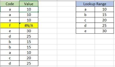
The highlighted cell has returned an error because it cannot find an exact match in the lookup range.

Here’s an example of where we’d use TRUE instead. Consider the below which has tables of sales and commission rates based on thresholds;

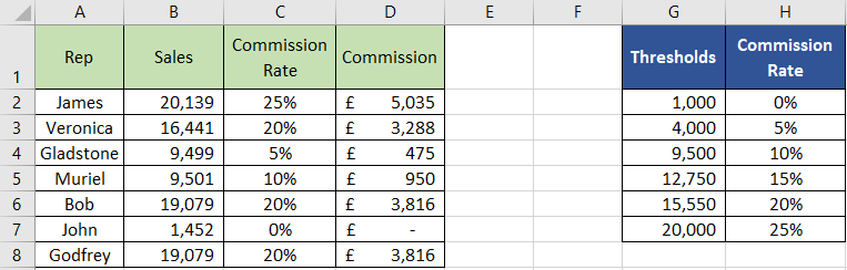
I want to lookup the value of Sales in the first table and return the appropriate commission percentage based on the thresholds in the second table.

So the formula in cell C2 is =VLOOKUP(B2,G1:H7,2, TRUE ). The value of Sales in B2 is 20,139 so it needs to do an approximate match which equates to 25% commission (good rates of commission at this company!). If we’d used FALSE, then the sales value would have to match exactly to that in the other table to return a value (i.e. 20,000).